|
Economía y Sociedad, Vol. 20, No 48 Cierre al 31 de diciembre del 2015, pp. 1-17 EISSN: 2215-3403 URL http://www.revistas.una.ac.cr/economia |
|
Economía y Sociedad, Vol. 20, No 48 Cierre al 31 de diciembre del 2015, pp. 1-17 EISSN: 2215-3403 URL http://www.revistas.una.ac.cr/economia |
PRODUCTION COSTS, PRICES AND INCOME OF FIRMS
COSTOS DE PRODUCCIÓN, PRECIOS E INGRESOS DE LA EMPRESA
Daniel Villalobos Céspedes1
Abstract
The present theoretical research analyzes microeconomic theory in regards to cost of production, prices, and firm’s revenue. We use simple mathematical tools to develop relationships of implied variables in the propounded model. The object of this is to explain microeconomic themes approximately to experiences of firms that produce a single good or service. It concludes that marginal cost and marginal revenue are not the most important factors in defining a firm’s equilibrium, but they are derived from the average cost and average revenue respectively. When consumer demand intensity and average profit rate are taken into consideration, the average cost and average revenue become fundamental concepts of theory cost and competition.
Keywords: resources; rate of profit; normal and extraordinary profits; market price.
Resumen
Esta investigación analiza la teoría microeconómica en relación con los costos de producción, precios e ingresos de las empresas. Se recurre a herramientas matemáticas simples para desarrollar las relaciones de las variables implicadas en el modelo propuesto. El objetivo es explicar los temas de modo aproximado a la experiencia de los empresarios. Se concluye que el costo marginal y el ingreso marginal, aunque derivados de los costos medios e ingresos medios respectivamente, no son los factores más importantes para la definición del equilibrio en una empresa en la industria. Cuando la intensidad de la demanda y la tasa media de ganancia son tomadas en cuenta, el costo medio y el ingreso medio constituyen conceptos fundamentales de la teoría de los costos y la competencia.
Palabras clave: recursos; tasa de ganancia; ganancias normales y extraordinarias; precio de mercado.
doi: http://dx.doi.org/10.15359/eys.20-48.1
Fecha de recepción: 06-08-15. Fechas de reenvíos: 14-09-2015/ 21-09-15.
Fecha de aceptación: 24-09-15. Fecha de publicación 14-10-15
I. Introduction
“To wherever that production goes, costs follow it as if it were a shadow” (Samuelson & Nordhaus 2010, p. 129). The phrase as if it were a shadow may be a misplaced metaphor. It may confuse an economics student, but it mainly encourages greater ignorance among firms. Production costs are the foundation of profitable activity and satisfying consumer needs. Costs are not hidden, but visible and essential; they are not mystical but instead manifestations of the production phenomenon. Costs establish the possibility of production because it is “the process of transforming inputs into outputs” and if we “want to consider firms producing only a single product from many inputs...it is more convenient to describe the firm’s technology in terms of a production function” (Jehle & Reny, 2001, p.119). Competitive rate of profit in an industry expresses the reality of production only if it is based on the costs of production. Firms’ costs are an intrinsic aspect of production options, and profits are greatly linked within it, highlighting the reality of production.
Rate of profit is the heart of production costs since it reflects opportunity costs. “Markets that work well, when all costs are included, the price is equal to the opportunity cost” (Samuelson and Nordhaus, 2010, p. 143). Competition evens out differences between firms in an industry, and thus, the profit rate is an average rate calculated from average costs in an industry. Firms that are highly or moderately efficient will be more or less competitive than an average firm in the industry. If all firms obtain normal profits, the market price would cover more than average production costs to be equal, or approximately equal, to opportunity costs. If the price of average efficiency companies rules the market in an industry, it is a consequence of the intensity of usual consumer demand (Marx 1986, Villalobos 2010). Therefore, the market price may be lower than the opportunity cost in less efficient companies and it will be higher in companies that are more efficient.
If the demand falls and the price of more efficient companies rules the market, less efficient and average firms will lose profits. In this case, the market price is lower than the cost of opportunity in less efficient and average firms, but this price could cover or slightly exceed average costs. In efficient companies, the market price would be equal to the opportunity cost, which would be reflected by obtaining a normal profit. If demand grows, in the short-term, the price of less efficient firms could prevail in the market. For these companies, the market price would be equal to the opportunity cost and they would make normal profits. However, medium and highly efficient companies might obtain abnormal or extraordinary profits since the price would be higher than the opportunity cost.
Average rate of profit is a competitive profit rate that will guide industry firms in the market. This rate is useful in calculating opportunity costs, because it defines a market price with reference to average industry costs and a given intensity of consumer demand. Average rate of profit prevents us from making the mistaken assumption that some costs are not taken into consideration for enterprises and that opportunity costs are the best alternative or discarded value. To enter into any industry, a firm assumes that the market price is the opportunity cost, which will be shown by normal or extraordinary profits or losses.
The comparative advantage concept is useful in describing opportunity costs among companies in the same industry. “The producer who has the smaller opportunity cost of producing a good is said to have a comparative advantage in producing that good” (Mankiw, 1998, p.52). Given the competitive profit rate in an industry and the typical demand in the market, a company with normal profits has a standard comparative advantage because the market price is equal to the opportunity cost. A firm with lower-than-average costs can obtain extraordinary profits and a greater comparative advantage since the market price is higher than its opportunity cost.
The purpose of this research paper is to provide a critical analysis of microeconomics. This study stems from concepts of “traditional” and “modern or advanced” microeconomics. Section II includes a review of the core microeconomics assumptions. Section III discusses total costs and production. Then in Section IV, the concepts of average and marginal costs are examined. Section V will analyze the rate of profits, prices, marginal cost, and marginal revenue, which will extend into Section VI. Lastly, following the conclusions, a list of references can be found.
II. Review of literature
Microeconomics usually begins by analyzing firms in terms of their production function. Call and Holahan (1983) justify production functions as “the cornerstone in the construction of the theory of the firm... In fact... [they] are the progenitor of the cost curves” (p.157). Based on the allocation of resources, it is presumed that there is a range of production functions between fixed and variable proportions (Samuelson, 1974; Ferguson, 1985; Varian. 1987; Ferguson & Gould, 1989; Call & Holahan, 1983; Bilas, 1993; Samuelson & Nordhaus, 2010; Mankiw, 1998; Jehle & Reny, 2001). According to these authors, production function is a matter of technical relationships established for production engineering. Production functions are complex since they involve a combination of inputs in the production of goods, services, and different kinds of products.
Key aspects of the theory of production are diminishing marginal product and the variable proportion of resources, which microeconomics gives character of law. This law describes that there is an increase in use intensity of fixed resources as variable ones are added. Intensity is synonymous with congestion or technical rigidity of fixed resources due to varying materials (Call & Holahan, 1983). This technical relationship is also of value as resources have prices in the market (Samuelson, 1974, Jehle & Reny, 2001).
Technical resource composition could reflect a relative decrease in the production level of employees, called marginal product of labor or diminishing average product of work. Diminishing marginal product refers to the physical relationship between the amount of output and use intensity of fixed resources. Fixed resources enter into the production process only one time and remain there according to use intensity during its useful life.2 During the useful life of a fixed resource, its use intensity involves a technical, efficient combination that tends to be optimal when variable resources are added (Ferguson & Gould, 1989). When production increases or decreases with a given fixed resource, use of other resources must increase or decrease as well (Jehle & Reny, 2001). The technical, efficient combination of resources does not change despite increasing or decreasing variable resources. Change in variable resources is necessary to achieve an efficient allocation of fixed resources.
A fixed resource has variable uses, making it possible to increase or decrease the use of other complementary and variable resources. If a fixed resource is partially unused, production could grow by intensifying its use and, of course, by increasing the quantity of variable resources (Marshall, 1895, Jehle & Reny, 2001).3 Optimal production of a fixed resource is possible if it is optimally combined with variable resources. Furthermore, a technical relationship of resources is a combination of resource value at market prices. If production increases or decreases, ceteris paribus, the value of combined resources could also increase or decrease due to varying prices. A technical combination of resources is stable, but a combined resource value is variable.
A fixed resource has unstable cost during its useful life, as its original cost will reduce according to the use intensity. Therefore, the fixed cost concept could vary in relation to the use intensity criterion. Therefore, the short-run definition must consider the fact that, in that period, the cost of fixed resources will decline as production increases. Producers are concerned for both technical and value combinations of resources. The average total cost of production fluctuates about regarding increases or decreases in the use of variable resources, given the use intensity of fixed resources. The greater the use intensity of fixed resources, the greater the use of variable resources and the lower the coefficient of resources value combination j will be.
In microeconomics, average fixed cost is the result of dividing total fixed cost value by quantity of output that a fixed resource helps generate. However, the fixed cost in any given moment of production is just a fraction of the value of fixed resources during their useful life. At any given time, only a small portion of the fixed resource value is transferred to the total product, and therefore only this portion enters into the computation of average fixed costs. Known as depreciation by Samuelson & Nordhaus (2010) and wear and tear by Marshall (1895), transferring fixed resource value to the product has an important role in figuring average costs and firm competitiveness.
Therefore, marginal cost refers to changes in the total cost of resources that arises from one extra unit of production. Fixed costs could be represented by property taxes, interest rates, leases, and implicit overhead costs. Nevertheless, it is common in economics to refer to the stock of fixed resources, which could include tangible and intangible .4 Ferguson & Gould (1989) commented in a footnote that the “short-run” is a well-defined length of time to adopt the analytical fiction that there is only a short-term. Then, supposing fixed resources as fixed value in the short-run is only fiction. We define a fixed resource as any resource that a firm must acquire to be used for long periods of production. Long-term is a more extended period of production, containing many short-runs. In long-run, the scale or size of firm’s plant will change.
Microeconomics assumes that the optimal level of production of a firm corresponds to the lowest-average, long-term total cost or equal marginal cost (Mankiw, 1998). Demand increase could raise profits if average costs are reduced and the scale of the plant is expanded. Demand intensity and competition could prevent a firm from investing in a new plant or expanding the current one due to the possibility of obtaining normal or abnormal profits. The demand for a product determines the quantity of that product a firm could sell, ceteris paribus, at market price bearing in mind the competition (Marshall, 1895).
A fundamental argument of microeconomics is that “combined income and the cost for the individual firm, and the demand and supply for all market, determine the market price and the production of the firm and the industry” (Ferguson & Gould, 1989, p. 225). In a competitive market, firms do not choose the price at which they sell their products; instead, they must face the market price at which they could sell the product (Marshall, 1895). Hayek (1967) first denied the influence of levels of prices on levels of production, but then he revised his position by considering the rate of profit (Hayek, 2002).
III. Total costs and production
Microeconomics defines total cost as the sum of fixed and variable costs.5 Suppose a firm is equipped with three sets of resources: fixed resources , circulating raw materials, inputs , and human resources . Resources of administration could be considered a special form of , such as management, furniture, stationery, logistics, intangible factors, among other fixed resources that affect the value combination of resources. Firms’ resources are measured according to their quantity and quality and are bought at market prices , and respectively. As Jehle & Reny (2001) explained:
“The firm’s cost of output is precisely the expenditure it must make to acquire the inputs used to produce that output. In general, the technology will permit every level of output to be produce by a variety of input vectors, and all such possibilities can be summarized by the level sets of the function production. The firm must decide, therefore, which of the possible production plans it will use. If the object of the firm is to maximize profits, it will necessarily choose the least costly, or cost-minimizing, production plan for every level of output…this will be true for all firms, whether monopolists, perfect competitors, or anything between” (p.126).
Total cost C of producing a good or service q with the set of resources K, T, Ç is defined as:
(1) C =PkK + Pc Ç + sT.
Every resource has an optimal technical level of combination determined by technology. Let k=Ç/K and therefore,
(2) Ç=kK.
Furthermore, if Ç is the total quantity necessary to produce a certain level of output q, then let ç=Ç/q. Thus, ç is the ration of Ç that a firm which minimizes costs must use for unit of output q. Hence,
(3) Ç = çq.
If equations (2) and (3) are equivalent, then
(4) çq = kK.
On the other hand, let t=K/T, so,
(5) K = t T.
If we insert equation (5) into equation (4), the result is
(6) çq = k t T.
By reorganizing equation (6) in relation to T, we obtain
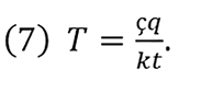
Then, by substituting equation (7) in equation (1), it now becomes
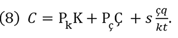
In equation (8), C is an added value of productive resources and its contribution is expressed at a level of q in accordance with a technical combination of values for a particular production process. This technical combination is set as an efficient and optimal physical fraction per unit of q. Value combination is given by the physical relationship and respective ratios of prices for resources. Let j be a ratio of value for fixed and circulating resources with respect to the value of human resources; furthermore, it expresses the intensity of resource value in the production process and can be expressed by equation (8) as
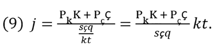
If pk=Pk /s and pc = Pc/s, we can substitute these expressions into equation (9) to obtain
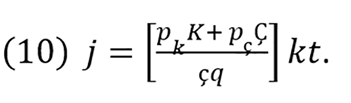
The influence of j on C is determined by reformulating equation (9) as
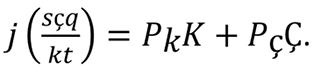
After replacing the left term in equation (8), the result is
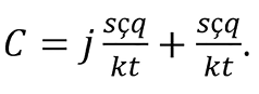
Consequently,
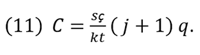
Equation (11) simplifies the expression of cost of production in terms of coefficients of resource combination at market value. Therefore, total costs are not just a simple sum of fixed and variable costs at each q- level.
IV. Average and Marginal Costs
By solving for q in equation (11), the average cost c is obtained as follows:
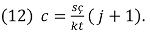
Equation (12) denotes that c is not a simple sum of average variable cost and average fixed cost. If q is rising, c tends to drop when j accelerates its fall, but it rises when j falls slowly and approaches the q- maximum. c is any average cost curve point called ci, where i = 1,2,3, ...n. Thus, qi indicates different q-levels for each ci. From equations (11) and (12), we know that C = cq, and therefore we can express
(13) Ci = ci qi .
C-changes are denoted as ΔC. We denote ΔC by equation (11):
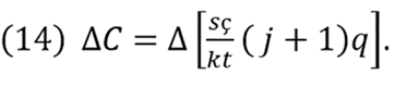
If we substitute equation (13) in equation (14), ΔC can be represented in a simplified form as
(15) ΔC = Δ(cq),
or by equation (15), ΔC can be shown between specific points on curve c as
(16) ΔC = Δ(ci qi).
The movement between these points is C1=c1 q1 and C2 = C1 + ΔC. Then, by operationalizing and replacing C1, we obtain ΔC = C2‒C1 = C2 ‒ c1 q1. Then, C2 = c2 q2. If we let c2 = c1 + Δc and q2 = q1 + Δq, thus ΔC = (c1 + Δc)(q1 + Δq) ‒ c1 q1 . Moreover, by operationalizing that equation, the result is ΔC = c1 q1+ c1 Δq + Δc q1 ‒ c1 q1, which can be simplified as ΔC=c1 Δq+Δc q1+Δc Δq. The resulting equation can now be expressed as
(17) ΔC = Δq (c1+Δc)+Δc q1 .
Having said that, the next sentence must be revised: “Although average total cost tells us the cost of the typical unit, it does not tell us how much total cost will change as the firm alters its level of production” (Mankiw, 1998; p. 272). As in microeconomics, marginal cost cm is the reason for changes in C and q, or it results from “the increase in total cost that arises from an extra unit of production” (Mankiw, 1998; p. 272). cm is derived from changes in equation (11), which is expressed in equation (17). Simply dividing both sides of equation (17) by Δq, or operating with Δq, and the result is
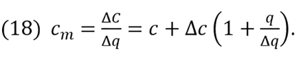
.
If in (18) Δq=0 and Δc<0, cm will infinitely decline, while it will infinitely increase if Δc>0. As q rises, initially cm<c , and then cm=c when c reaches the minimum, and from that point on, cm> c. These general relationships are best expressed by leveling equation (18) to equation (12), where cm = c. So,
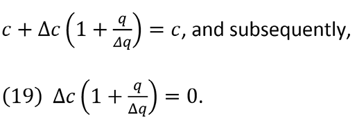
Equation (19) indicates that the point in which cm ≈ c, where c, cm curve intersects q-axis and c and cm curves will overlap. At this point, firms earn normal profits as Im ≈ Ime. When c, cm curve is placed in the negative quadrant, cm < c, and when it is in the positive quadrant, cm > c.
V. Rate of Profits, Prices, Marginal Cost, and Marginal Revenue
Let ρ denote market average price per unit of q, where I = ρq represents the total value of -level of output or the company’s total income I. That price is given by equation (11) supposing average rate of profit ġ is defined by competition and other market conditions. As a result,
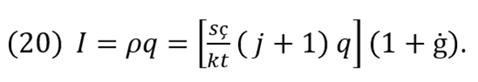
By operationalizing equation (20) in term of q, we obtain
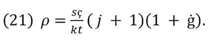
The first term on the right side of equation (21) is c as defined in equation (12); therefore, by simplifying, we can substitute it, resulting in
(22) ρ = c (1+ġ).
Changes between two points in I is defined as ΔI, which is produced by changes in ρ and q, denoted Δρ and Δq, respectively. Changes in ρ and q are motivated by a variation in components of c, ġ, or both. If there are Δρ, ceteris paribus, it will necessarily be reflected as ġ-changes, denoted Δġ.
If I1=ρ1 q1=c1 (1+ġ1)q1 and, I2= ρ2 q2=c2 (1+ġ2) q2
where ρ2 = ρ1 + Δρ, q2=q1 + Δq, c2 =c1+ Δc, and ġ2 = ġ1+ Δġ,
then we can say that
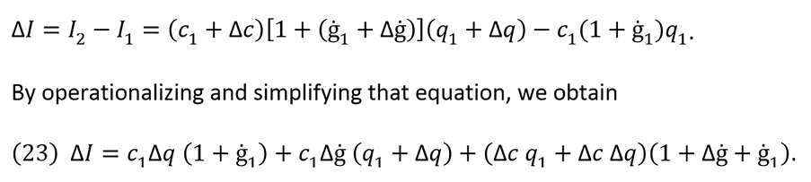
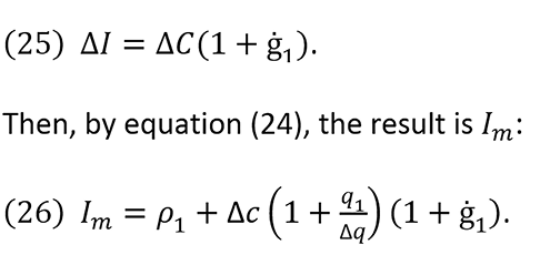
In microeconomics, marginal revenue Im is defined, in a simplified mathematical procedure, as the ratio of ΔI and Δq, shown as Im=ΔI/Δq. If we operationalize equation (23) and simplify according to Δq, the result is
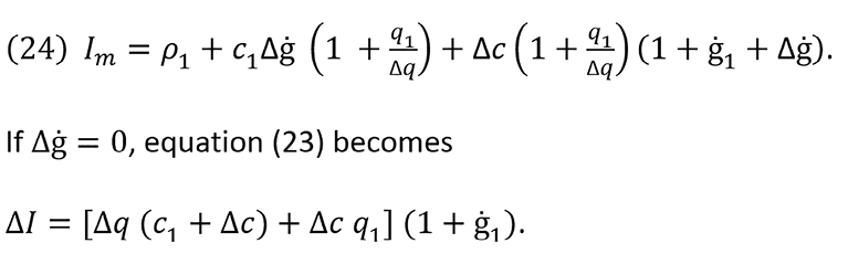
According to equation (17), the first term on the right side of the previous equation is ΔC. Therefore, we can substitute it and obtain
A general equation to determine relationships between Im and cm for each q-level is given by dividing both sides of equation (25) by Δq, resulting in
(27) Im= cm (1+ġ).
or by equation (26),
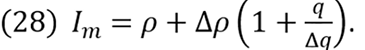
If in equation (28) Δq = 0 and Δρ < 0, Im will infinitely decline, while it will infinitely increase if Δρ > 0. Thus, Im > cm if and only if ġ > 0.
VI. Income, Marginal Revenue, and Marginal Cost
Average income Ime is defined as
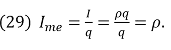
In equation (22), I can be represented in general terms as
I = c(1+ġ)q.
From which follows
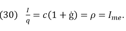
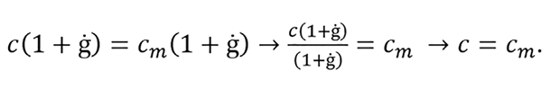
The relationship between ρ, Ime, and Im comes from equations (27) and (30), shown as
c(1+ġ) = cm (1+ġ)→ ρ = Im .
and also
If c = cm, then Im = Ime and firms earn normal profits at ġ > 0.6 Below this, c > cm and Ime>Im , and firms will have losses at ġ > 0. Above it, c < cm and Ime < Im , and, ceteris paribus, firms could still obtain normal profits. Only in a possible case where ġ = 0 can it be said that c = cm = Im = Ime = ρ at some q-level. If ġ > 0, it is always true that Im> cm for any known q-level. There is a common point where cm = Ime, which represents the firm’s equilibrium at a given level of consumer demand. A company has a range of q-suboptimal where c = cm, or its equivalent Im = Ime. What is below this range reaches a q-minimum, which would imply the leaving point of a company from the industry, until q obtains equilibrium at cm = Ime Ime. Anything above this range could shrink the average profit. This scenario could happen because (Im‒ cm )=ġcm = (Ime‒c)=ġc, or the marginal profit is equal to the average profit ġcm = ġc at q-optimal.
Let the average rate of profit in the industry be
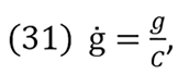
And therefore,
(32) g=ġC.
For any movement, such as g1 to g2 or vice versa, the change in g, denoted Δg, can be given by Δq, ΔC or Δġ which results from changes in ΔPk, ΔPç , Δs usual demand intensity, tax rates, technology, interest rates, or use intensity of K and T, for instance added overtime, more working days, among other factors.
If
(33) g1=ġ1 C1, and
(34) g2=ġ2 C2, and
(35) ġ2=ġ1+Δġ,
We can substitute equation (35) in equation (34) to obtain
(36) g2 = (ġ1+Δġ) C2.
Then,
(37) C2=C1+ΔC.
By inserting equation (37) into equation (36), the result is
(38) g2=(ġ1+Δġ) (C1+ΔC).
Now if
(39) Δg = g2 ‒ g1,
We can substitute equations (32) and (36) into equation (39) to obtain
Δg = (ġ1+Δġ)(C1+ΔC) ‒ ġ1 C1 .
By operationalizing the equation,
Δg = ġ1 C1+ ġ1 ΔC+ΔġC1+Δġ ΔC ‒ ġ1 C1 ,
And after simplifying, it becomes
Δg = ġ1 ΔC + ΔġC1 + Δġ ΔC.
Then, the resulting equation is
(40) Δg=ġ1 ΔC + Δġ (C1+ΔC).
If Δġ = 0, subsequently,
(41) Δg = ġ1 ΔC.
By substituting equation (17) in equation (41), we obtain
(42) Δg = ġ1 [Δq (c1 + Δc) + Δcq1].
After dividing both sides of equation (42) by Δq, the outcome is marginal profit gm, represented as
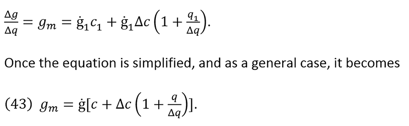
From equations (18), it is known that
(44) gm = ġcm
Equation (44) is retained in equation (27) and ġ1c2 would be given by equation (30). Hence, Im : cm : Ime : c at a given g; that is, Im is to as Ime is to cm at a given ġ. Above the q-equilibrium, a company could obtain normal or abnormal profits as the usual demand becomes more intense. Ceteris paribus, this scenario is possible due to the idle capacity in K-firm. If demand is relatively higher than usual and there is K-idle capacity in a firm, greater investment in K could result in a higher opportunity cost.
VII. Conclusions
Fixed resources enter the production process at a specific time and will remain there as the use intensity consumes its economic useful life. During that time, the use intensity implies some efficient technical combination that may be optimal when variable resources are added (Ferguson and Gould 1989). When production increases or decreases with a given fixed resource, variable resources will as well. On the other hand, the technical combination of resources remains constant despite an increase or decrease in other resources.
Fixed resources have varying uses, making it possible to increase or decrease the use of other resources. If fixed resources are partially idle, production can be increased by expanding their use, which requires a greater amount of variable resources. Optimal production of a single fixed resource is possible when an increase or decrease in other resources ceases. This technical relationship involves a value resource combination for market prices. When production increases or decreases given the technical combination of resources, the combined resource value will also increase or decrease.
The technical combination of resources is an average measure while its combined value is variable. Fixed resources are acquired at market price, which is a cost for the firm. However, during its useful life, fixed resources have variable costs regarding its use intensity. For this very reason, average fixed costs will vary during the production period. Therefore, in the production process, technical resource combination and resources value are important. Given the use intensity of fixed resources, the average cost of production changes as the use of variable resources fluctuates. As the use intensity of fixed resources increases, the quantity of variable resources must grow and the combined resources value will drop.
A growing demand could allow firms to grow their profits if increasing supply reduces average cost of output. A firm should expand the scale of its plant and perhaps, to invest in new technology in this case. Intensity demand and competition will guide firms in spending new investments. In the short-run, firms could have idle fixed resources that could be used in case of a rising demand. Firms do not expand production until their profits reach a maximum. Firms increase production to a level at which losses are minimized or to where they could have normal or extraordinary profits. When marginal revenue is equal to the average income, firms can maintain operations, but it will incur losses if the profit rate becomes zero.
The average revenue curve is the firm’s supply curve, which indicates the competitive market price at which the firm could sell its product in accordance with its average cost for each level of production and its average profit rate. A firm will be in balance only when it obtains normal profits, considering the usual demand and competitive price governing the market. Nevertheless, a firm could obtain normal or extraordinary profits when, ceteris paribus, demand is too intense at the price ruling the market.
New research can use this theoretical result to study competition and firm competitiveness. We consider this to be a new approach to old microeconomic concepts that could open minds when studying a firm’s behavior.
References
Bilas, R. A. (1993). Teoría Microeconómica. Retrieved from https://books.google.co.cr/books/about/Teor%C3%ADa_microecon%C3%B3mica.html?id=DBqOrs43m00C&redir_esc=y
Call, S. T., Holahan, L. W. (1983). Microeconomía. Retrieved from https://books.google.co.cr/books/about/Microeconom%C3%ADa.html?id=GHljQgAACAAJ&redir_esc=y
Ferguson, C. E., Gould, J. P. (1989). Teoría Microeconómica. Retrieved from http://www.fondodeculturaeconomica.com/Librerias/Catalogo.aspx?buscar=Teor%C3%ADa+Microecon%C3%B3mica&cat=ofefep
Ferguson, C. E. (1985). Teoría Neoclásica de la Producción y la Distribución. México: Editorial Trillas.
Hayek, F. A. (1967). Prices and Production (2 ed). Retrieved from https://books.google.co.cr/books/about/Prices_and_Production.html?id=K5PUAAAAMAAJ&redir_esc=y
Hayek, F.A. (1975). “Profits, Interest and Investment: and other essays on the theory of industrial fluctuations”. Retrieved from https://books.google.co.cr/books/about/Profits_interest_and_investment.html?id=n9wOAQAAMAAJ&redir_esc=y
Hayek, F. A. (2002). “Competition as a Discovery Procedure” (Translation by Marcellus, S. S). The Quarterly Journal of Austrian Economics, 5(3), 9-23. Retrieved from http://link.springer.com/article/10.1007/s12113-002-1029-0
Jehle, A. G., Reny, J. P. (2001). Advanced Microeconomic Theory. Retrieved from https://books.google.co.cr/books/about/Advanced_Microeconomic_Theory.html?id=_RS3AAAAIAAJ&redir_esc=y
Mankiw, N. G. (1998). Principles of Microeconomics. Retrieved from https://books.google.co.cr/books/about/Principles_of_Microeconomics.html?id=xoztFMavGCcC&redir_esc=y
Marshall, A. (1985). Principles of Economics. Retrieved from https://books.google.co.cr/books/about/Principles_of_Economics.html?id=bykoAAAAYAAJ&redir_esc=y
Marx, K. (1986). El Capital: Libro Tercero: El Proceso Global de la Producción Capitalista.Retrieved from https://books.google.co.cr/books/about/El_capital_Libro_tercero_El_proceso_glob.html?id=WrjQrQEACAAJ&redir_esc=y
Samuelson, P. A. (1974). Curso de Economía Moderna. Retrieved from https://books.google.co.cr/books/about/Curso_de_econom%C3%ADa_moderna.html?id=RGNUPQAACAAJ&redir_esc=y
Samuelson, P. A., Nordhaus, W. D. (2010). Microeconomía con Aplicaciones a América Latina. Retrieved from http://www.mheducation.com.mx/9786071503343-latam-macroeconomia-con-aplicaciones-a-america-latina
Varian, H. R. (1987). Intermediate Microeconomics: A Modern Approach. Retrieved from https://books.google.co.cr/books/about/Intermediate_Microeconomics.html?id=kcCoW-oUSJoC&redir_esc=y
Villalobos, D.C. (2010). Capital, Competencia y Ganancia. Retrieved from http://www.euna.una.ac.cr/index.php/100-categorias/lineas-editoriales/ciencias-sociales/134-capital-competencia-y-ganancia
Notas:
1 Economista, politólogo, académico Universidad de Costa Rica (UCR) y Universidad Nacional de Costa Rica (UNA). Correo electrónico danielvillalobosc@gmail.com; daniel.villalobos.cespedes@una.cr
2 Microeconomics defines fixed costs as “costs that do not vary with the quantity of output produced” (Mankiw, 1998). This is called short-run, a time horizon in which a firm cannot adjust the number or sizes of it factory. However, it is just a rigid assumption, because in short-term, fixed resources varied their value according the amount of output by considering depreciation.
3 Marginal cost and marginal product are possible if, and only if, some fixed resources are idle or “is not being used” (Mankiw, 1998). Marginal cost of a marginal product will drop because of the use intensity of fixed resources but, ceteris paribus, it will rise as variable resources are added.
4 Capital is “a generic term that represents all of the fixed factors” (Call and Holahan, 1983, p.199). Nevertheless, capital is also understood in the sense of useful effects of resources, such as production and profits.
5 Bilas (1993) wrote in a footnote, “The plant can be defined as a group of buildings that house a higher or lower quantity of fixed assets.” (p. 205). Regarding time-term Ferguson and Gould (1989) point out that “the definition of long-term is reasonably clear: It is a period of time long-enough for what all inputs it totally adjusting; a short term is a more nebulous concept.”” (p. 188)). Thus, long-term is a less hazy concept and therefore reasonably clearer than the short-term concept.
6 Microeconomics points out that, in these circumstances, a firm will get profits equal to zero;, and below it is a leaving point.

Revista Economía y Sociedad by Universidad Nacional is licensed under a Creative Commons Reconocimiento-NoComercial-CompartirIgual 4.0 Internacional License.
Creado a partir de la obra en http://www.revistas.una.ac.cr/index.php/economia.